Overview of Basic MOSViz Functionality
MOSViz is composed of separate components that interact via “linked views.” As described below, and as shown in Figures 1, MOSViz includes a:
- 1D spectral viewer
- 2D spectral viewer
- Image cutout viewer
- Data table
- 2D scatter plot
- 3D scatter plot, and a
- mosaic viewer where the targets are indicated.
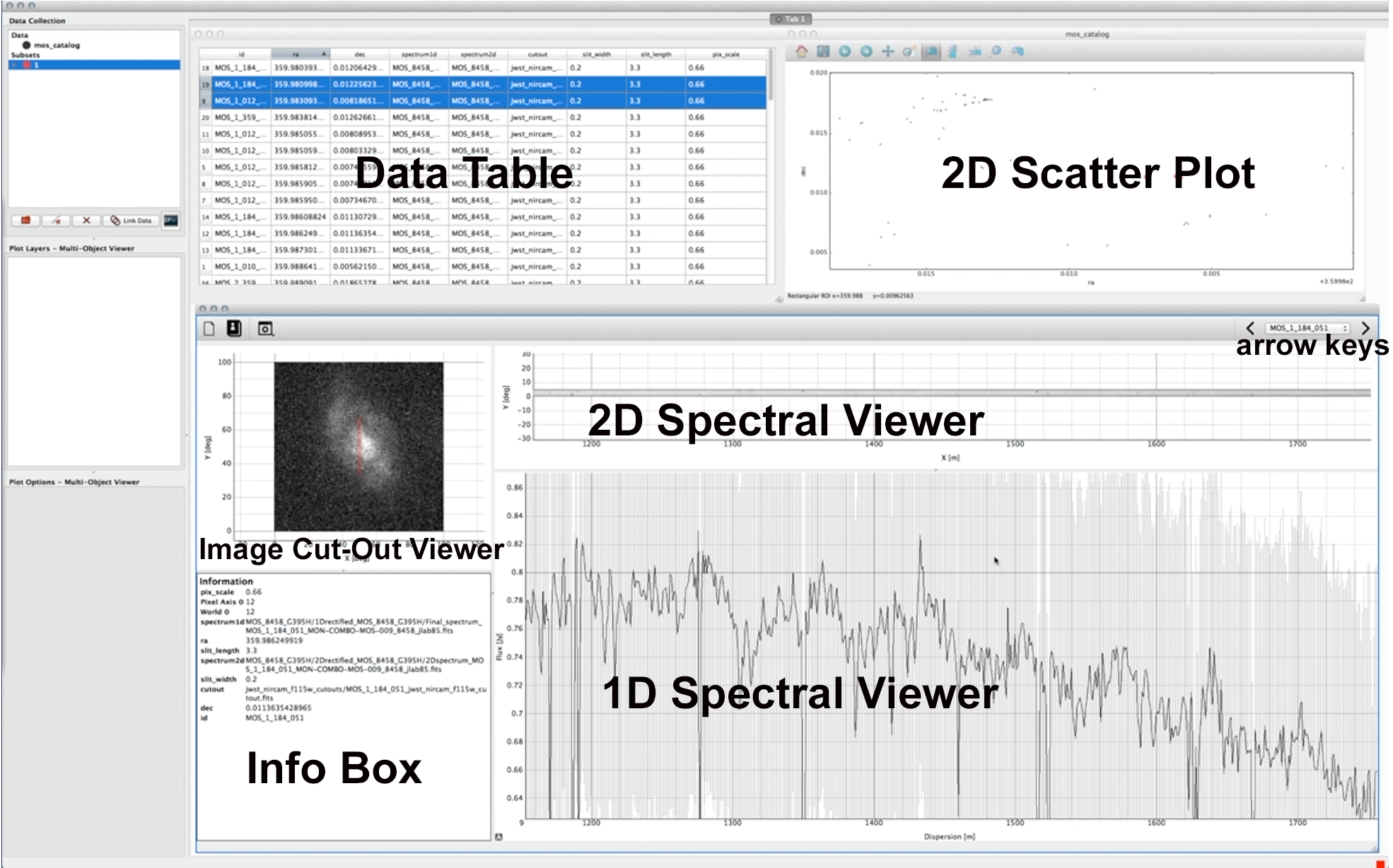
Figure 1: A screen shot of MOSViz with its components labeled is shown. MOSViz is embedded in the Glue visualization tool. In the use case shown, the user has selected targets in the scatter plot on the upper right. The corresponding rows in the table are highlighted, and the first object’s 1D and 2D spectra are shown. The cutout image has the spectral aperture indicated on it in red. The user advances to the next target in the spectra/image viewers by hitting the arrow key in the upper right. Shown in the MOS viewer is a simulated NIRCam image and an “engineering” NIRSpec MSA spectrum with faked errors.
Each of these components is described in more detail below. Once a MOS data set is read in, users can use any combination of these tools. A typical use case/workflow is the following:
- Read in a table of: target identifications, coordinates (RA, DEC), paths and file names of cutout images, paths and file names of 2D spectra, paths and file names of 1D spectra, and optional quantities (such as star-formation rate magnitudes, stellar masses, sizes, etc.) for 1000 galaxies at a redshift of 2
- Sort galaxies in table according to star-formation rate
- Highlight the 3 galaxies with the highest star-formation rates
- This causes the 1D and 2D spectra and cut-out image of the first galaxy of these three galaxies to display
- Measure the equivalent width of an emission line
- Hit the arrow button to move to the next galaxy
- Do the same for the second and third objects
MOSViz’s main purpose is to help users to visually inspect and perform a “first-look” analysis of multiple spectra. To this end, MOSViz’s main component is its 1D and 2D spectral viewers. The user can choose to use both 1D and 2D viewers, or either one. Users can interact further with the 1D spectra by opening the SpecViz 1D spectral analysis tool. SpecViz allows users to make measurements of e.g, emission and absorption line strengths and sky continuum levels. For the 2D spectra, a basic set of view adjustments will is available: zoom, pan, colormap, and intensity scaling.
MOSViz also includes an optional cutout viewer to show an image of each target alongside their 1D and 2D spectra. The cutout is aligned so that the cross-dispersion direction has the same vertical orientation as for the 2D spectrum. We provide documentation on how to create such cutouts for single-waveband images and multi-band color images. For the single-waveband cutouts, a basic set of view adjustments will be available in future versions of MOSViz: zoom, pan, colormap, and intensity scaling. The UI will read back the row, column and flux under in the pixel under the cursor. In addition, we provide documentation on how to show overlayed spectral apertures on each cutout image (at above link). For most MOS’s, the spectral aperture is a thin slit. For the NIRSpec MSA, it is a single or multi-shutter “slitlet”.
MOSViz’s default is to lock the wavelength axis of the 1D and 2D spectra so that they are aligned spatially and zoom and pan together. It also defaults to have the cross-dispersion spatial axis locked to the cutout vertical axis so that they zoom and pan together. All of the data must have valid WCSs for this to work.
The data table allows users to select targets to display in the spectral and/or cutout viewers. Optionally, they can also display the selected targets in the 2D and/or 3D scatter plots and/or on the large image viewer (the latter available in future versionsof MOSViz). Columns in the data table must include at minimum target identification (id), right ascension (RA), and declination (DEC). The table can include any other quantities the user wishes to include. Its columns can be sorted. The user can select as many or as few objects as they wish to view.
The optional 2D and 3D scatter plots can be used to plot the quantities in the tables. The user can click on each point/target in the plots to display the selected target’s spectra and images. The user can select multiple contiguous points/targets at once.
Finally, the information box displays the information from the table on the specific target displayed.