Reading-in Data

MOSViz will be able to read in NIRSpec MSA data straight from the pipeline or archive. This will include 1D and 2D spectra, images, data tables, and associated images. This page documents how to read in MOS data from another observatory. An example is shown at the bottom (Defining custom readers for spectra and cutouts).

The general workflow can be summarized as follows:

1. Start Glue by typing glue in the command line
2. In Glue, click on the folder icon and open the file containing the Data Table for your data set.
3. Drag the file from the Data Collection window into the main canvas.
4. Select ‘MOSViz Viewer’ from the pop-up menu.
5. Use the green arrow buttons at the top of the viewer to switch between objects.

Overview

MOSViz requires at minimum the following input:

• A catalog of targets in tabular form
• A 1D and 2D spectrum for each target
• A cutout image for each target

The main data file that will be read in and used by the MOSViz viewer is the catalog. The catalog can be in any format that Glue understands (such as a FITS table, VO table, ASCII table, and so on). The main constraint is that the table should include columns with the following information for each target:

Column	Default name	Units
File path to the 1D spectrum	spectrum1d
File path to the 2D spectrum	spectrum2d
File path to the image cutout	cutout
Right ascension of the slit center (FK5 J2000)	ra	degrees
Declination of the slit center (FK5 J2000)	dec	degrees
Width of the slit	slit_width	arcseconds
Length of the slit	slit_length	arcseconds

The columns can have any name, but if they are given the name in the Default name column above, they will be automatically recognized. In addition, the catalog can contain any other useful information such as source names, magnitudes, stellar masses, star-formation rates, etc. These are not required, but including them will allow selections to be done on those parameters.

When adding a dataset to the MOSViz viewer for the first time in glue, the following dialog will appear:

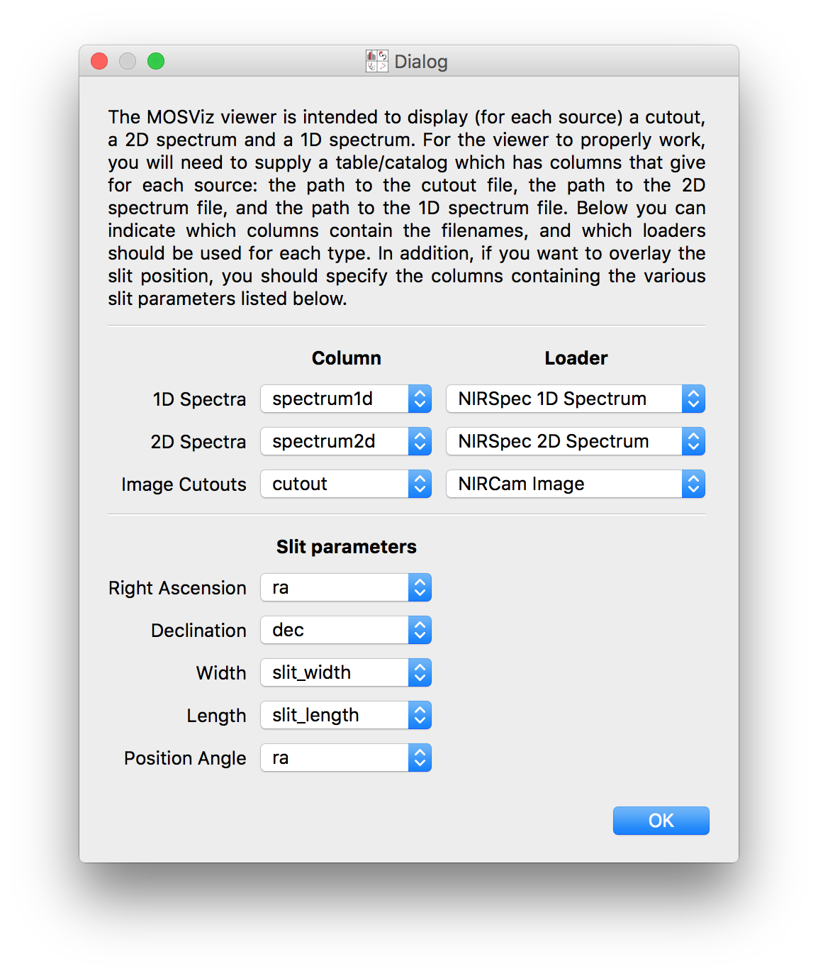
This dialog asks to confirm the column names and also asks to select the appropriate readers for the 1D and 2D spectra as well as the cutouts. In Defining custom readers for spectra and cutouts we show how to define custom readers for spectra and cutouts in case there isn’t an appropriate built-in reader available, and in Writing the Data Table we show how to tell MOSViz which readers/columns to use by default.

Defining custom readers for spectra and cutouts

This example uses spectra and cutout images of galaxies at 0.2<z<1.2 which have spectra from the DEIMOS multi-object spectrograph on Keck and color cut-out images already created from Hubble/ACS. These galaxies are from the DEEP2 Survey. The spectra can be obtained from the DEEP2 Data Release page.

MOSViz is a Glue plugin so we’ll write our own Custom Data Loaders to read data. All we need to do is write a function which takes a filename as input and returns a glue Data object. For this example, we have three different types of data: a 1D Spectrum, a 2D spectrum, and a cutout image.

1D Spectrum Reader

MOSViz expects the 1D Spectrum Data object to have three components: Wavelength, Flux, and Uncertainty. The final reader we are going to write is as follows:

from astropy.io import fits
from glue.core import Data
from mosviz.loaders.mos_loaders import mosviz_spectrum1d_loader

@mosviz_spectrum1d_loader('DEIMOS 1D Spectrum')
def deimos_spectrum1D_reader(filename):
    """
    Data loader for Keck/DEIMOS 1D spectra.

    This loads the 'Bxspf-B' (extension 1) and 'Bxspf-R' (extension 2) and
    appends them together to proudce the combined Red/Blue Spectrum along
    with their Wavelength and Inverse Variance arrays.
    """

    hdulist = fits.open(filename)
    data = Data(label='1D Spectrum')
    data.header = hdulist[1].header

    full_wl = np.append(hdulist[1].data['LAMBDA'][0], hdulist[2].data['LAMBDA'][0])
    full_spec = np.append(hdulist[1].data['SPEC'][0], hdulist[2].data['SPEC'][0])
    full_ivar = np.append(hdulist[1].data['IVAR'][0], hdulist[2].data['IVAR'][0])

    data.add_component(full_wl, 'Wavelength')
    data.add_component(full_spec, 'Flux')
    data.add_component(1/np.sqrt(full_ivar), 'Uncertainty')

    return data

Let’s take a look at how to write this step by step. We first take a look at the contents of our example FITS file to see which parts we need to pass to MOSViz:

>>> from astropy.io import fits
>>> hdulist = fits.open('spec1d.1355.134.13040873.fits')
>>> hdulist.info()
Filename: spec1d.1355.134.13040873.fits
No.    Name         Type      Cards   Dimensions   Format
  0  PRIMARY     PrimaryHDU       4   ()
  1  Bxspf-B     BinTableHDU    131   1R x 15C   [4096E, 4096E, 4096E, 4096I, 4096I, 4096I, 4096I, 4096I, E, E, E, J, J, 4096E, E]
  2  Bxspf-R     BinTableHDU    131   1R x 15C   [4096E, 4096E, 4096E, 4096I, 4096I, 4096I, 4096I, 4096I, E, E, E, J, J, 4096E, E]
  3  Horne-B     BinTableHDU    140   1R x 15C   [4096E, 4096E, 4096E, 4096I, 4096I, 4096I, 4096I, 4096I, E, E, E, J, J, 4096E, E]
  4  Horne-R     BinTableHDU    140   1R x 15C   [4096E, 4096E, 4096E, 4096I, 4096I, 4096I, 4096I, 4096I, E, E, E, J, J, 4096E, E]
  5  Bxspf-NL-B  BinTableHDU    131   1R x 15C   [4096E, 4096E, 4096E, 4096I, 4096I, 4096I, 4096I, 4096I, E, E, E, J, J, 4096E, E]
  6  Bxspf-NL-R  BinTableHDU    131   1R x 15C   [4096E, 4096E, 4096E, 4096I, 4096I, 4096I, 4096I, 4096I, E, E, E, J, J, 4096E, E]
  7  Horne-NL-B  BinTableHDU    140   1R x 15C   [4096E, 4096E, 4096E, 4096I, 4096I, 4096I, 4096I, 4096I, E, E, E, J, J, 4096E, E]
  8  Horne-NL-R  BinTableHDU    140   1R x 15C   [4096E, 4096E, 4096E, 4096I, 4096I, 4096I, 4096I, 4096I, E, E, E, J, J, 4096E, E]

The file contains pairs of red and blue spectra which have been filtered in various ways. For the sake of this example we’ll choose the Bxspf spectra. Let’s take a closer look at the relevant extension:

>>> hdulist['Bxspf-R'].columns
ColDefs(
    name = 'SPEC'; format = '4096E'
    name = 'LAMBDA'; format = '4096E'
    name = 'IVAR'; format = '4096E'
    name = 'CRMASK'; format = '4096I'
    name = 'BITMASK'; format = '4096I'
    name = 'ORMASK'; format = '4096I'
    name = 'NBADPIX'; format = '4096I'
    name = 'INFOMASK'; format = '4096I'
    name = 'OBJPOS'; format = 'E'
    name = 'FWHM'; format = 'E'
    name = 'NSIGMA'; format = 'E'
    name = 'R1'; format = 'J'
    name = 'R2'; format = 'J'
    name = 'SKYSPEC'; format = '4096E'
    name = 'IVARFUDGE'; format = 'E'
)
>>> hdulist['Bxspf-B'].columns
ColDefs(
    name = 'SPEC'; format = '4096E'
    name = 'LAMBDA'; format = '4096E'
    name = 'IVAR'; format = '4096E'
    name = 'CRMASK'; format = '4096I'
    name = 'BITMASK'; format = '4096I'
    name = 'ORMASK'; format = '4096I'
    name = 'NBADPIX'; format = '4096I'
    name = 'INFOMASK'; format = '4096I'
    name = 'OBJPOS'; format = 'E'
    name = 'FWHM'; format = 'E'
    name = 'NSIGMA'; format = 'E'
    name = 'R1'; format = 'J'
    name = 'R2'; format = 'J'
    name = 'SKYSPEC'; format = '4096E'
    name = 'IVARFUDGE'; format = 'E'
)

Again, there are a lot of options but for MOSViz we’re only interested in three columns: SPEC, LAMBDA, IVAR. Further, MOSViz expects each of the arrays to be 1 dimensional and of the same size:

>>> hdulist['Bxspf-R'].data['SPEC'].shape
(1, 4096)
>>> hdulist['Bxspf-R'].data['LAMBDA'].shape
(1, 4096)
>>> hdulist['Bxspf-R'].data['IVAR'].shape
(1, 4096)

All of our arrays are the same size but they are stored in 2 dimensional arrays (with the first axis of size 1). So we’ll just take the first (and only) element.

Now that we know what data we want from our FITS files let’s look at how to write the data loader function. The basic structure for a data loader for a 1D spectrum is:

from glue.core import Data
from mosviz.loaders.mos_loaders import mosviz_spectrum1d_loader

@mosviz_spectrum1d_loader('DEIMOS 1D Spectrum')
def deimos_spectrum1D_reader(filename):
    # code to read in data here
    return data

'DEIMOS 1D Spectrum' is the label which is how we will identify this loader. For users familiar with defining glue data factories, @mosviz_spectrum1d_loader is equivalent to @data_factory but additionaly tells MOSViz that the loader is specifically for a 1D spectrum.

Let’s now focus on what is needed inside the function. The function itself takes a filename to open as its only argument, so we open the file and instantiate a Glue Data object:

hdulist = fits.open(filename)
data = Data(label='1D Spectrum')

Now as above we’re going to open the FITS file. We add the header from the FITS file to the data object:

data.header = hdulist[1].header

As stated above, MOSViz expects the Wavelength, Flux, and Uncertainty to be each be a single 1D array. We saw that the red and blue ends of the spectrum are stored in different extensions and that there are stored as 2D arrays. We take the first component of the each of the red and blue ends of the spectrum and combine them together. Then we take the full 1D array for each component and pass them to the ~glue.core.data.Data object using the add_component() method:

full_wl = np.append(hdulist[1].data['LAMBDA'][0], hdulist[2].data['LAMBDA'][0])
full_spec = np.append(hdulist[1].data['SPEC'][0], hdulist[2].data['SPEC'][0])
full_ivar = np.append(hdulist[1].data['IVAR'][0], hdulist[2].data['IVAR'][0])

data.add_component(full_wl, 'Wavelength')
data.add_component(full_spec, 'Flux')
data.add_component(1/np.sqrt(full_ivar), 'Uncertainty')

return data

2D Spectrum Reader

The basic structure for the 2D spectrum reader is similar to that for the 1D spectrum reader:

from astropy.io import fits
from glue.core import Data
from mosviz.loaders.mos_loaders import mosviz_spectrum1d_loader

@mosviz_spectrum2d_loader('DEIMOS 2D Spectrum')
def deimos_spectrum2D_reader(filename):
    """
    Data loader for Keck/DEIMOS 2D spectra.

    This loads only the Flux and Inverse variance. Wavelength information
    comes from the WCS.
    """

    hdulist = fits.open(filename)
    data = Data(label='2D Spectrum')
    data.coords = coordinates_from_header(hdulist[1].header)
    data.header = hdulist[1].header
    data.add_component(hdulist[1].data['FLUX'][0], 'Flux')
    data.add_component(1/np.sqrt(hdulist[1].data['IVAR'][0]), 'Uncertainty')
    return data

MOSViz expects the 2D Spectrum Data object to have two components: Flux and Uncertainty. Since a 2D spectrum is an image it also expects a World Coordinate System (WCS) which tells it how to transform from pixels to Wavelength. Let’s take a look at the contents of our example FITS file to see which parts we need to pass to MOSViz:

>>> from astropy.io import fits
>>> hdulist = fits.open('slit.1355.134B.fits.gz')
>>> hdulist.info()
Filename: slit.1153.147B.fits.gz
No.    Name         Type      Cards   Dimensions   Format
0    PRIMARY     PrimaryHDU       4   ()
1    slit        BinTableHDU    106   1R x 11C     [241664E, 241664E, 241664B, 241664B, 4096E, 241664E, 6D, 3D, 59E, 177E, 241664J]
2    slit        BinTableHDU     98   531R x 5C    [E, E, E, E, B]
>>> hdulist[1].data.columns
ColDefs(
    name = 'FLUX'; format = '241664E'; dim = '( 4096, 59)'
    name = 'IVAR'; format = '241664E'; dim = '( 4096, 59)'
    name = 'MASK'; format = '241664B'; dim = '( 4096, 59)'
    name = 'CRMASK'; format = '241664B'; dim = '( 4096, 59)'
    name = 'LAMBDA0'; format = '4096E'
    name = 'DLAMBDA'; format = '241664E'; dim = '( 4096, 59)'
    name = 'LAMBDAX'; format = '6D'
    name = 'TILTX'; format = '3D'
    name = 'SLITFN'; format = '59E'
    name = 'DLAM'; format = '177E'; dim = '( 59, 3)'
    name = 'INFOMASK'; format = '241664J'; dim = '( 4096, 59)'
)
>>> hdulist[2].data.columns
ColDefs(
    name = 'AMP'; format = 'E'
    name = 'CEN'; format = 'E'
    name = 'SIG'; format = 'E'
    name = 'BASE'; format = 'E'
    name = 'MASK'; format = 'B'
)

MOSViz needs Flux and Uncertainty so the relevant columns are FLUX and IVAR in the the first slit extension:

>>> hdulist[1].data['FLUX'].shape
(1, 59, 4096)
>>> hdulist[1].data['IVAR'].shape
(1, 59, 4096)
>>>

All of our arrays are the same size but they are stored in 3 dimensional arrays (with the first axis of size 1). So we’ll just take the first (and only) element which will give a 2D array.

We also need a WCS which should be in the header of the same extension as the data:

>>> from astropy.wcs import WCS
>>> WCS(hdulist[1].header)

Number of WCS axes: 2
CTYPE : 'LAMBDA'  'LAMBDA'
CRVAL : 6450.6538154  0.0
CRPIX : 0.0  0.0
CD1_1 CD1_2  : 0.32103118300400002  0.0
CD2_1 CD2_2  : 0.0  1.0
NAXIS    : 4367352 1

The WCS is here; however, the two axes both have name ‘LAMBDA’ and if we look at look at the second coordinate we can see that it isn’t actually transformed. Glue expects that all of a Data object’s components (including WCS axes) have unique names. We can take care of this easily in the data loader function.

Now that we know what data we want from our FITS files let’s look at how to write the data loader function. As before, we use the following decorator to tell glue that this is a data loader, and MOSViz that it can read in 2D spectra:

@mosviz_spectrum2d_loader('DEIMOS 2D Spectrum')
def deimos_spectrum2D_reader(filename):

The function itself takes a filename to open as its only argument. We open the data file and instantiate a Data object:

hdulist = fits.open(filename)
data = Data(label='2D Spectrum')

As we noted above, the WCS axes should have different names. Since the second axis is not transformed we’ll just change the header keyword which specifies its name to ‘Spatial Y’ Then we set the coords attribute of the Data object with glue.core.coordinates.coordinates_from_wcs(). We also pass the FITS header to the data so that useful information can be displayed in the MOSViz:

hdulist[1].header['CTYPE2'] = 'Spatial Y'
data.coords = coordinates_from_wcs(WCS(hdulist[1].header))
data.header = hdulist[1].header

As stated above, MOSViz expects the Flux and Uncertainty to be each be a single 2D array. We take the first component of each array (a 2D array) pass them to the ~glue.core.data.Data object using the add_component() method:

data.add_component(hdulist[1].data['FLUX'][0], 'Flux')
data.add_component(1/np.sqrt(hdulist[1].data['IVAR'][0]), 'Uncertainty')

return data

Cutout Image Reader

Finally, the custom reader for the image cutouts looks like:

from astropy.io import fits
from glue.core import Data
from mosviz.loaders.mos_loaders import mosviz_cutout_loader

@mosviz_cutout_loader('ACS Cutout Image')
def acs_cutout_image_reader(filename):
    """
    Data loader for the ACS cut-outs for the DEIMOS spectra.

    The cutouts contain only the image.
    """

    hdulist = fits.open(filename)
    data = Data(label='ACS Cutout Image')
    data.coords = coordinates_from_header(hdulist[0].header)
    data.header = hdulist[0].header
    data.add_component(hdulist[0].data, 'Flux')

    return data

MOSViz expects the Cutout Image Data object to have one component: Flux. Since it is an image it also expects a World Coordinate System (WCS) which tells it how to transform from pixels to sky coordinates. Let’s take a look at the contents of our example FITS file to see which parts we need to pass to MOSViz.

>>> from astropy.io import fits
>>> hdulist = fits.open('12020821.acs.i_6ac_.fits')
>>> hdulist.info()
Filename: 12020821.acs.i_6ac_.fits
No.    Name         Type      Cards   Dimensions   Format
0    PRIMARY     PrimaryHDU      71   (201, 201)   float32
>>> hdulist[0].data.shape
(201, 201)

There is only one extensions and the data in it is the cutout image (a 2D array). We also need a WCS which should be in the header of the same extension as the data:

>>> from astropy.wcs import WCS
>>> WCS(hdulist[0].header)
WCS Keywords

Number of WCS axes: 2
CTYPE : 'RA---TAN'  'DEC--TAN'
CRVAL : 214.40388488799999  52.630077362100003
CRPIX : 101.70472905800101  100.94206076200101
CD1_1 CD1_2  : -8.3333331279300006e-06  -4.5781947460699999e-14
CD2_1 CD2_2  : -4.5781947460699999e-14  8.3333331279300006e-06
NAXIS    : 201 201

The WCS looks as we would expect. Now that we know what data we want from our FITS files let’s look at how to write the data loader function. We use the following decorator on the function to tell glue that this is a data factory and to tell MOSViz that it can handle cutout images:

@mosviz_cutout_loader('ACS Cutout Image')
def acs_cutout_image(filename):

The function itself takes a filename to open as its only argument. We open the data file and instantiate a Data object:

hdulist = fits.open(filename)
data = Data(label='Cutout Image')

We set the coords attribute of the Data object with glue.core.coordinates.coordinates_from_wcs(). We also pass the FITS header to the data so that useful information can be displayed in the MOSViz:

data.coords = coordinates_from_wcs(WCS(hdulist[0].header))
data.header = hdulist[0].header

We take the data in first extension data array (a 2D array) and pass it to the ~glue.core.data.Data object using the add_component() method:

data.add_component(hdulist[0].data, 'Flux')

return data

Summary

The full contents of the ~/.glue/config.py is shown below:

import numpy as np

from astropy.io import fits
from astropy.wcs import WCS

from glue.core import Data
from glue.core.coordinates import coordinates_from_header, coordinates_from_wcs

from mosviz.loaders.mos_loaders import (mosviz_spectrum1d_loader,
                                        mosviz_spectrum2d_loader,
                                        mosviz_cutout_loader)


@mosviz_spectrum1d_loader('DEIMOS 1D Spectrum')
def deimos_spectrum1D_reader(filename):
    """
    Data loader for Keck/DEIMOS 1D spectra.

    This loads the 'Bxspf-B' (extension 1)
    and 'Bxspf-R' (extension 2) and appends them
    together to proudce the combined Red/Blue Spectrum
    along with their Wavelength and Inverse Variance
    arrays.
    """

    hdulist = fits.open(filename)
    data = Data(label='1D Spectrum')
    data.header = hdulist[1].header

    full_wl = np.append(hdulist[1].data['LAMBDA'][0], hdulist[2].data['LAMBDA'][0])
    full_spec = np.append(hdulist[1].data['SPEC'][0], hdulist[2].data['SPEC'][0])
    full_ivar = np.append(hdulist[1].data['IVAR'][0], hdulist[2].data['IVAR'][0])

    data.add_component(full_wl, 'Wavelength')
    data.add_component(full_spec, 'Flux')
    data.add_component(1/np.sqrt(full_ivar), 'Uncertainty')

    return data

@mosviz_spectrum2d_loader('DEIMOS 2D Spectrum')
def deimos_spectrum2D_reader(filename):
    """
    Data loader for Keck/DEIMOS 2D spectra.

    This loads only the Flux and Inverse variance.
    Wavelength information comes from the WCS.
    """

    hdulist = fits.open(filename)
    data = Data(label='2D Spectrum')
    data.coords = coordinates_from_header(hdulist[1].header)
    data.header = hdulist[1].header
    data.add_component(hdulist[1].data['FLUX'][0], 'Flux')
    data.add_component(1/np.sqrt(hdulist[1].data['IVAR'][0]), 'Uncertainty')
    return data

@mosviz_cutout_loader('ACS Cutout Image')
def acs_cutout_image_reader(filename):
    """
    Data loader for the ACS cut-outs for the DEIMOS spectra.

    The cutouts contain only the image.
    """

    hdulist = fits.open(filename)
    data = Data(label='ACS Cutout Image')
    data.coords = coordinates_from_header(hdulist[0].header)
    data.header = hdulist[0].header
    data.add_component(hdulist[0].data, 'Flux')

    return data

Writing the Data Table

As mentioned above, when adding a dataset to the MOSViz viewer, you will be prompted to select column names and data loaders, but you can optionally encode these into the catalog metadata to save time. Note that not all file formats will support this kind of meta-data, so if you want to do this you will be restricted to certain formats for the catalog.

The main requirement is that when read in with the Table read() method, the Table meta attribute should be a dictionary that contains a loaders key and a special_columns key:

• Table.meta['loaders'] should then be a dictionary that contains three keys - spectrum1d, spectrum2d, and cutout, and for each of these gives, as a string, the label of the reader to use.
• Table.meta['special_columns'] should be a dictionary that contains one key/value pair for each special column listed in the table in Overview, where the key is the Default name given in the table and the value is the name of the actual column in the table.

Note that any metadata where the defaults are fine can be omitted. For example, for the special columns, if the actual name is the same as the default name, the key and value will be the same and can be ommitted from the metadata.

As an example, the following ECSV table header indicates the loaders to use, but does not list the special columns explicitly since they already have the expected names:

# %ECSV 0.9
# ---
# meta:
#   loaders:
#       spectrum1d: "DEIMOS 1D Spectrum"
#       spectrum2d: "DEIMOS 2D Spectrum"
#       cutout: "ACS Cutout Image"
# datatype:
# - {name: id, datatype: string}
# - {name: ra, unit: deg, datatype: float64}
# - {name: dec, unit: deg, datatype: float64}
# - {name: spectrum2d, datatype: string}
# - {name: spectrum1d, datatype: string}
# - {name: cutout, datatype: string}
# - {name: slit_width, unit: arcsec, datatype: float64}
# - {name: slit_length, unit: arcsec, datatype: float64}
# - {name: pix_scale, datatype: float64}
id ra dec spectrum2d spectrum1d cutout slit_width slit_length pix_scale
deimos_12004808 214.21968 52.410386 Spectra/slit.1153.151R.fits.gz Spectra/spec1d.1153.151.12004808.fits Cutouts/12004808.acs.v_6ac_.fits 0.2 3.3 0.0 0.66
deimos_12008179 214.33785 52.454369 Spectra/slit.1203.063R.fits.gz Spectra/spec1d.1203.063.12008179.fits Cutouts/12008179.acs.v_6ac_.fits 0.2 3.3 0.0 0.66
deimos_12012573 214.34313 52.53112  Spectra/slit.1205.091R.fits.gz Spectra/spec1d.1205.091.12012573.fits Cutouts/12012573.acs.v_6ac_.fits 0.2 3.3 0.0 0.66
deimos_12016058 214.52242 52.580972 Spectra/slit.1208.055R.fits.gz Spectra/spec1d.1208.055.12016058.fits Cutouts/12016058.acs.v_6ac_.fits 0.2 3.3 0.0 0.66
deimos_12020734 214.49056 52.632246 Spectra/slit.1209.080R.fits.gz Spectra/spec1d.1209.080.12020734.fits Cutouts/12020734.acs.v_6ac_.fits 0.2 3.3 0.0 0.66
deimos_12020387 214.57266 52.642585 Spectra/slit.1210.072R.fits.gz Spectra/spec1d.1210.072.12020387.fits Cutouts/12020387.acs.v_6ac_.fits 0.2 3.3 0.0 0.66
deimos_12020049 214.62085 52.646039 Spectra/slit.1211.061R.fits.gz Spectra/spec1d.1211.061.12020049.fits Cutouts/12020049.acs.v_6ac_.fits 0.2 3.3 0.0 0.66
deimos_12019995 214.69602 52.631649 Spectra/slit.1212.038R.fits.gz Spectra/spec1d.1212.038.12019995.fits Cutouts/12019995.acs.v_6ac_.fits 0.2 3.3 0.0 0.66
deimos_12019653 214.77361 52.662353 Spectra/slit.1214.026R.fits.gz Spectra/spec1d.1214.026.12019653.fits Cutouts/12019653.acs.v_6ac_.fits 0.2 3.3 0.0 0.66
deimos_12008349 214.249   52.460424 Spectra/slit.1243.030R.fits.gz Spectra/spec1d.1243.030.12008349.fits Cutouts/12008349.acs.v_6ac_.fits 0.2 3.3 0.0 0.66
deimos_12012586 214.37004 52.52134  Spectra/slit.1243.079R.fits.gz Spectra/spec1d.1243.079.12012586.fits Cutouts/12012586.acs.v_6ac_.fits 0.2 3.3 0.0 0.66
deimos_12004455 214.27608 52.408039 Spectra/slit.1244.010R.fits.gz Spectra/spec1d.1244.010.12004455.fits Cutouts/12004455.acs.v_6ac_.fits 0.2 3.3 0.0 0.66
deimos_11051203 214.33513 52.381078 Spectra/slit.1246.011R.fits.gz Spectra/spec1d.1246.011.11051203.fits Cutouts/11051203.acs.v_6ac_.fits 0.2 3.3 0.0 0.66
deimos_12011504 214.61256 52.551567 Spectra/slit.1246.152R.fits.gz Spectra/spec1d.1246.152.12011504.fits Cutouts/12011504.acs.v_6ac_.fits 0.2 3.3 0.0 0.66
deimos_12024856 214.5929  52.718354 Spectra/slit.1252.066R.fits.gz Spectra/spec1d.1252.066.12024856.fits Cutouts/12024856.acs.v_6ac_.fits 0.2 3.3 0.0 0.66
deimos_13004306 214.77715 52.814133 Spectra/slit.1253.152R.fits.gz Spectra/spec1d.1253.152.13004306.fits Cutouts/13004306.acs.v_6ac_.fits 0.2 3.3 0.0 0.66
deimos_12024118 214.73955 52.697049 Spectra/slit.1254.094R.fits.gz Spectra/spec1d.1254.094.12024118.fits Cutouts/12024118.acs.v_6ac_.fits 0.2 3.3 0.0 0.66
deimos_12020067 214.64333 52.632145 Spectra/slit.1255.041R.fits.gz Spectra/spec1d.1255.041.12020067.fits Cutouts/12020067.acs.v_6ac_.fits 0.2 3.3 0.0 0.66
deimos_13019968 214.77751 52.910775 Spectra/slit.1302.115R.fits.gz Spectra/spec1d.1302.115.13019968.fits Cutouts/13019968.acs.v_6ac_.fits 0.2 3.3 0.0 0.66
deimos_13026888 215.01438 52.949334 Spectra/slit.1306.072R.fits.gz Spectra/spec1d.1306.072.13026888.fits Cutouts/13026888.acs.v_6ac_.fits 0.2 3.3 0.0 0.66
deimos_13026873 215.0064  52.95921  Spectra/slit.1306.077R.fits.gz Spectra/spec1d.1306.077.13026873.fits Cutouts/13026873.acs.v_6ac_.fits 0.2 3.3 0.0 0.66
deimos_13026857 214.95442 52.969926 Spectra/slit.1306.094R.fits.gz Spectra/spec1d.1306.094.13026857.fits Cutouts/13026857.acs.v_6ac_.fits 0.2 3.3 0.0 0.66
deimos_13026107 215.10585 53.003483 Spectra/slit.1308.070R.fits.gz Spectra/spec1d.1308.070.13026107.fits Cutouts/13026107.acs.v_6ac_.fits 0.2 3.3 0.0 0.66
deimos_13025290 215.19495 52.963721 Spectra/slit.1309.034R.fits.gz Spectra/spec1d.1309.034.13025290.fits Cutouts/13025290.acs.v_6ac_.fits 0.2 3.3 0.0 0.66
deimos_13043017 215.10605 53.116245 Spectra/slit.1311.114R.fits.gz Spectra/spec1d.1311.114.13043017.fits Cutouts/13043017.acs.v_6ac_.fits 0.2 3.3 0.0 0.66
deimos_13051276 215.10065 53.128093 Spectra/slit.1311.121R.fits.gz Spectra/spec1d.1311.121.13051276.fits Cutouts/13051276.acs.v_6ac_.fits 0.2 3.3 0.0 0.66
deimos_13041627 215.31852 53.104803 Spectra/slit.1313.048R.fits.gz Spectra/spec1d.1313.048.13041627.fits Cutouts/13041627.acs.v_6ac_.fits 0.2 3.3 0.0 0.66
deimos_13050572 215.17647 53.154515 Spectra/slit.1313.104R.fits.gz Spectra/spec1d.1313.104.13050572.fits Cutouts/13050572.acs.v_6ac_.fits 0.2 3.3 0.0 0.66
deimos_13050507 215.14259 53.169163 Spectra/slit.1313.120R.fits.gz Spectra/spec1d.1313.120.13050507.fits Cutouts/13050507.acs.v_6ac_.fits 0.2 3.3 0.0 0.66
deimos_13058235 215.23847 53.184374 Spectra/slit.1314.098R.fits.gz Spectra/spec1d.1314.098.13058235.fits Cutouts/13058235.acs.v_6ac_.fits 0.2 3.3 0.0 0.66
deimos_13049212 215.38783 53.136419 Spectra/slit.1315.047R.fits.gz Spectra/spec1d.1315.047.13049212.fits Cutouts/13049212.acs.v_6ac_.fits 0.2 3.3 0.0 0.66
deimos_13049133 215.3953  53.156244 Spectra/slit.1315.052R.fits.gz Spectra/spec1d.1315.052.13049133.fits Cutouts/13049133.acs.v_6ac_.fits 0.2 3.3 0.0 0.66
deimos_13058203 215.27553 53.210001 Spectra/slit.1315.105R.fits.gz Spectra/spec1d.1315.105.13058203.fits Cutouts/13058203.acs.v_6ac_.fits 0.2 3.3 0.0 0.66
deimos_13018671 214.95738 52.921481 Spectra/slit.1343.084R.fits.gz Spectra/spec1d.1343.084.13018671.fits Cutouts/13018671.acs.v_6ac_.fits 0.2 3.3 0.0 0.66
deimos_13026879 215.00536 52.95371  Spectra/slit.1343.108R.fits.gz Spectra/spec1d.1343.108.13026879.fits Cutouts/13026879.acs.v_6ac_.fits 0.2 3.3 0.0 0.66
deimos_13034580 215.08674 53.055397 Spectra/slit.1352.022R.fits.gz Spectra/spec1d.1352.022.13034580.fits Cutouts/13034580.acs.v_6ac_.fits 0.2 3.3 0.0 0.66
deimos_13058164 215.26445 53.18501  Spectra/slit.1352.117R.fits.gz Spectra/spec1d.1352.117.13058164.fits Cutouts/13058164.acs.v_6ac_.fits 0.2 3.3 0.0 0.66
deimos_13040952 215.32582 53.068148 Spectra/slit.1355.091R.fits.gz Spectra/spec1d.1355.091.13040952.fits Cutouts/13040952.acs.v_6ac_.fits 0.2 3.3 0.0 0.66
deimos_13040873 215.40401 53.11767  Spectra/slit.1355.134R.fits.gz Spectra/spec1d.1355.134.13040873.fits Cutouts/13040873.acs.v_6ac_.fits 0.2 3.3 0.0 0.66

If the ra/dec columns had a different name in the table, the header should instead look like e.g:

# %ECSV 0.9
# ---
# meta:
#   loaders:
#       spectrum1d: "DEIMOS 1D Spectrum"
#       spectrum2d: "DEIMOS 2D Spectrum"
#       cutout: "ACS Cutout Image"
#   special_columns:
#       ra: ra_j2000
#       dec: dec_j2000
# datatype:
# - {name: id, datatype: string}
# - {name: ra_j2000, unit: deg, datatype: float64}
# - {name: dec_j2000, unit: deg, datatype: float64}
...